Title of Slides

Lecture \(n\) - CODE10001

Placeholder

This slide is split into two columns, one with a list and one with an image from the web.

  1. List item A,
  2. List item B,
  3. List item C,
  4. Final list item.

Two square panels show identical sets of scattered black dots, with only the red additions being different. The left panel shows a slightly rising red line drawn through the middle of the panel, passing near a few dots but not obviously related to most of them. A red text is below the dots: R-squared = 0.06. The right panel shows many of the dots connected by red lines to form a stick figure of a man resembling the constellation Orion, with the hand on the reader's right raised and holding an object. A red text is below the dots: Rexthor, the Dog-Bearer. A caption is below and spanning both panels: I don't trust linear regressions when it's harder to guess the direction of the correlation from the scatter plot than to find new constellations on it.

xkcd.com/1725, Randall Munroe (2016) CC BY-NC 2.5.

To access the speaker notes for these slides, tap s on your keyboard.

To export the slides, tap e and then print to PDF.

Example Section

Maths

Equations are formatted with \(\mathrm{\LaTeX}\), either inline with $...$ or centred with $$...$$.

Theorem: Quadratic Equation

If \(ax^2 + bx + c = 0\) where \(a\neq0\), then the solutions are given by \(x = \frac{-b \pm \sqrt{b^2 - 4ac}}{2a}\).

Proof

\[\begin{align} ax^2 + bx + c &= 0 \\ 4a^2 x^2 + 4abx + 4ac &= 0 \\ 4a^2 x^2 + 4abx + b^2 &= b^2 - 4ac \\ {(2ax + b)}^2 &= b^2 - 4ac \\ 2ax + b &= \pm\sqrt{b^2 - 4ac} \\ 2ax &= -b\pm\sqrt{b^2 - 4ac} \\ x &= \frac{-b\pm\sqrt{b^2 - 4ac}}{2a} \\ \end{align}\]

Note

This is Śrīdhara’s method. The steps of the derivation are:

  1. Multiply both sides by \(4a\).
  2. Add \(b^2 - 4ac\) to both sides.
  3. Complete the square on the left hand side.
  4. Take the square root of both sides.
  5. Subtract \(b\) from both sides.
  6. Divide both sides by \(2a\) (since \(a\neq0\)). \(\square\)

Nice Plots

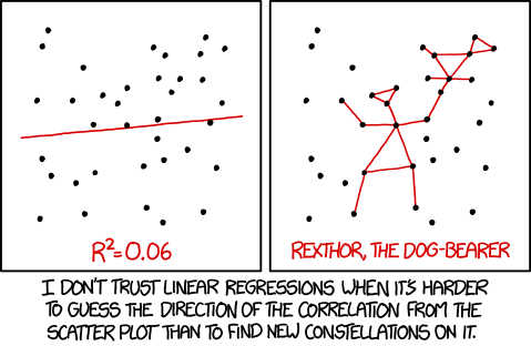
Given response \(y\) and single predictor \(x\), this model fits to the equation

\[\begin{equation} y = \beta_{0} + \beta_{1}x. \end{equation}\]

Visually, the line of best fit from linear regression may look like the below.

Scatter diagram for the classic 'mtcars' dataset, showing miles per gallon against horsepower. A linear regression of y = 30 - 0.068x is shown.

Code Output

If we roll a dice 30 times, how many threes would we expect to get?

Theoretical Outcome

The \(\mathbb{P}(X=3) = \frac{1}{6}\). Therefore we expect to get \(30\times\frac{1}{6} = 5\) threes.

In practice, it probably won’t be exactly that many.

# sample space is dice face values
faces <- c(1, 2, 3, 4, 5, 6)

# roll it 30 times, allow repeats
rolls <- sample(faces, 30, replace=TRUE)

# display outcomes as a chart and a list
hist(rolls, breaks=0:6); rolls

 [1] 3 1 3 2 6 1 4 5 5 3 6 2 1 1 5 3 1 6 1 6 4 6 2 4 1 2 4 1 4 5